ROI Pop-Up Menu

Opens the Dataset Cropper panel. In this panel you can crop an ROI (see Cropping Datasets).

Opens the Dataset Sampler panel. In this panel you can modify spacing by upsampling or downsampling (see Sampling Datasets).

Opens the Dataset Inverter panel. In this panel you can invert the labeled voxels within a region of interest (see Inverting Datasets).

Opens the Dataset Properties panel. The basic and advanced properties related to an ROI can be viewed and modified here (see Dataset Properties).

Generates a contour mesh that describes the surface of a region of interest (see Generating Contour Meshes from ROIs).

Opens the Object Description dialog, in which you can add a description to the selected object or edit its current description.

Lets you create a graph of a region of interest, which can provide a ready-made framework for performing a wide range of pore network simulations to better understand how porous materials behave and how to improve them (see Graphing Regions of Interest).

Automatically creates a multi-ROI in which the segments contained within the selected region of interest are labeled as separate connected components. You should note that segments are determined by first skeletonizing the region of interest, applying a watershed, and then expanding the ROI and assigning a label to each branch.

The computed multi-ROI will appear as a new item in the Data Properties and Settings panel. (see Graphing Multi-ROIs).

Exports the selected ROI in the ORS Object file format (*.ORSObject extension). ORS files are proprietary binary formatted files in which data is written sequentially and XML (Extensible Markup Language) is appended after the binary data (see Exporting Objects).

Exported regions of interest can be reloaded to continue a segmentation or to maintain consistency between related datasets.

Exports the basic properties of the selected ROI and its statistical properties in the CSV file format. The basic properties of an ROI include its name, T index, total voxel count, labeled voxel count, and other parameters. The statistical properties of an ROI can include the volume of labeled voxels, percentage volume, surface, and Feret diameters, as well as the min, max, mean, and standard deviation of an associated dataset.

Exports the basic properties of the selected ROI and its statistical properties in the GDT1 file format. The basic properties of an ROI include its name, T index, total voxel count, labeled voxel count, and other parameters. The statistical properties of an ROI can include the volume of labeled voxels, percentage volume, surface, and Feret diameters, as well as the min, max, mean, and standard deviation of an associated dataset.

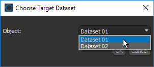
Exports the selected region of interest to a series of image files (TIFF, JPEG, BMP, or PNG file formats), as raw data, or in the ORSObject file format (*.ORSObject), in which labeled voxels are assigned a value of 1 and all other voxels 0. The geometry of the exported files can be selected in the Choose a Target Dataset dialog, as shown below.

Lets Dragonfly Pro users export ROIs in the CZI file format (*.czi extensioni). CZI is a proprietary file format used by ZEISS microscopes to save data.

Provides a shortcut for selecting macros that can be executed for a single ROI.

Automatically creates a new connectivity multi-ROI, in which each group of connected voxels is labeled as a distinct object. In the 6-connected scheme, the propagation of connected components is done by strictly using the 6 faces adjacent to the current seed and will result in the maximum number of labeled objects (see Connectivity).

Automatically creates a new connectivity multi-ROI, in which each group of connected voxels is labeled as a distinct object. In the 26-connected scheme, the propagation of connected components is done in all directions using the 6 faces, 12 edges, and 8 corners adjacent to the current seed and will result in the fewest number of labeled objects (see Connectivity).

Creates a new connectivity multi-ROI and opens the Object Analysis dialog, in which you can further analyze the multi-ROI. See Quantification for information about analyzing the connected components in a multi-ROI.

Copies the selected region of interest and adds it to the Data Properties and Settings panel.

Saves the selected region of interest as a template (see ROI Templates).

Allows you to save reformations, such as oblique and double-obliques, that were applied with the Walk tool and other methods. The result is a new region of interest formatted in the current space (see Creating Oblique Views).

Automatically rotates the selected ROI so that the selected axis is aligned to the Z-axis of the world coordinate system.

Automatically aligns the centroid of the selected region of interest with the centroid of another object. Applicable objects include volumetric image data, regions of interest, multi-ROIs, and meshes. Reference objects can be selected in the Choose the object to align with dialog, shown below.

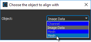
The centroid of a region of interest is calculated from the bounding box that encapsulates the labeled voxels of the ROI. It is not calculated from its geometry.

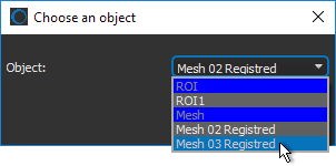
Automatically applies transformations, such as translations and rotations, that were applied to a reference object to the selected region of interest.

You should note that only objects that were previously transformed will be available as a reference in the Choose an object dialog, shown below.

Automatically identifies region of interest segments as connected and non-connected porosity (see Connected Porosity).

NOTE This feature is available for Dragonfly Pro only.

The Process Islands options — Remove or Isolate by voxel count or rank — let you refine thresholded segmentation results or isolate objects of a certain size (see Processing Islands).

Plots a histogram of the selected region of interest with the values of a selected dataset (see Region of Interest Histograms).

Lets you minimize beam hardening effects.

Lets to close inner holes smaller than a selected threshold distance. Threshold distances are selectable in the Threshold dialog.

Creates a new multi-ROI, in which the labeled voxels of each selected ROI is labeled as a distinct object. For example, if you create a multi-ROI from five regions of interest, then the multi-ROI will contain five labels.

Lets you compute the degree of anisotropy for the selected region of interest using the mean intercept length (MIL) method (see Computing Anisotropy).

Lets you compute the degree of anisotropy for the selected region of interest using the star volume distribution (SVD) method (see Computing Anisotropy).

Creates a distance map from the selected ROI (see Creating Distance Maps).

Creates a signed distance map from the selected ROI (see Creating Distance Maps).

Lets you reduce each connected component in a region of interest to a single-voxel wide skeleton, as shown below.

Original ROI (green) and skeletonized ROI (red)

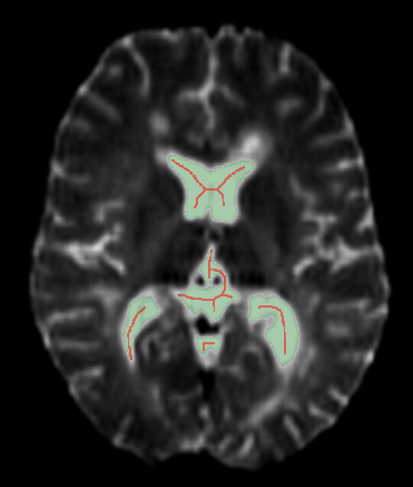
For best results, any inner holes in the region of interest must be filled (see How to Fill Inner Areas).

Automatically computes local thickness for each point in the selected region of interest. You should note that computations are based on the sphere-fitting method and that local thickness is defined as the diameter of the largest sphere which fulfills two conditions:

• The sphere encloses the point, but the point is not necessarily in the center of the sphere.
• The sphere is entirely bounding within the solid surfaces of the region of interest.

Creates a geodesic distance map in which the shortest path from a seed point that joins all points inside a region of interest are mapped. You should note that LUTs can be applied to geodesic distance maps, which can be examined in 2D and 3D views and are computed using the Fast Marching method.

Geodesic distance map of a pore network

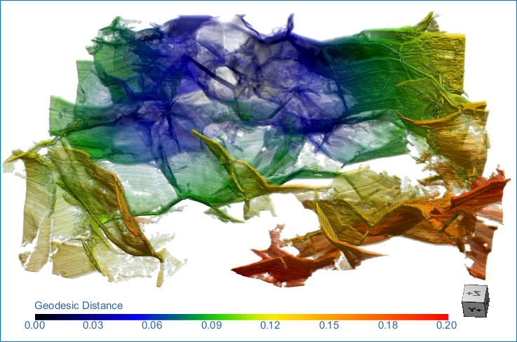
To create a geodesic distance, right-click the region of interest that you need to map and then choose Create Geodesic Distance Map in the pop-up menu. You can then select the seed point in the Choose a Seed ROI dialog.

The geodesic distance is the shortest path fully contained within a region that joins two points, while the Euclidean distance is the straight line distance.

Lets you automatically align the axis of inertia of the selected region of interest with the axis of inertia of another ROI.

Generates a convex hull as a filled region of interest for the selected ROI (see Generating Convex Hulls).

Generates a convex hull as an outlined region of interest for the selected ROI (see Generating Convex Hulls).

Generates a convex hull as a mesh for the selected ROI (see Generating Convex Hulls).

Automatically crops the region of interest to the bounding box that encapsulates the labeled voxels of the ROI.

Automatically aligns the center of mass of the selected region of interest in the current 2D scene views. You should note that the center of mass is calculated from the labeled voxels within the bounding box of the ROI.

Automatically removes objects, which can be defined as groups of labeled voxels that are connected, within the current region of interest that intersect with a selected ROI or multi-ROI.

In the example below, the objects in the ROI with the orange circles that were touching the blue ROI were removed.

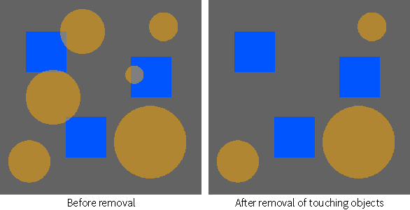
• Right-click the region of interest you need to modify and then choose Remove Objects That Touch Another ROI or Multi-ROI in the pop-up menu.
• Choose the ROI or multi-ROI that is touching parts of the region of interest that you are modifying in the Choose ROI or Multi-ROI dialog.

  

• Click OK.

  Touching objects are removed automatically from the selected ROI.

Creates a new region of interest that contains only labeled voxels with an original neighbor count greater than or equal to a selected threshold. Thresholds are selectable in the Neighbor Count dialog, shown below.

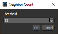
This option is often used in the topological analysis of skeletons.

Automatically creates a box that corresponds to the dimensions of the labeled voxels in the selected region of interest.

Automatically creates a box that corresponds to the dimensions of the labeled and unlabeled voxels in the selected region of interest.

Copies the intersected values of the selected object(s) into the geometry (or shape) of another object to create a new dataset. Might be necessary if you need to extract statistics from an ROI or multi-ROI, such as the minimum, maximum, or mean values of corresponding image data (see Statistical Properties), or intend to compute other measures that require consistent shapes.

• Enter a new name for the sampled object in the Name field.
• Choose the object with the required geometry in the Geometry drop-down menu.

  

• Click OK.

  The intersected values are copied into the new shape and the resulting object appears in the Data Properties and Settings panel.

Exports each selected region of interest in the ORS Object file format (*.ORSObject extension) to a separate file (see Exporting Objects).

If the selected regions of interest share the same name, their file names will be appended with a sequential number.

Exports the selected regions of interest in the ORS Object File (*.ORSObject extension) to a single file (see Exporting Objects).

Exports the basic properties of the selected ROIs and their statistical properties in the GDT 1 file format. The basic properties of an ROI include its name, T index, total voxel count, labeled voxel count, and other parameters. The statistical properties of an ROI can include the volume of labeled voxels, percentage volume, surface, and Feret diameters, as well as the min, max, mean, and standard deviation of an associated dataset.

Exports the selected regions of interest to a series of image files (TIFF, JPEG, BMP, or PNG file formats), as raw data, or in the ORSObject file format (*.ORSObject), in which labeled voxels are assigned a value of 1 and all other voxels 0. The geometry of the exported files can be selected in the Choose a Target Dataset dialog, as shown below.

Lets Dragonfly Pro users export ROIs in the CZI file format (*.czi extensioni). CZI is a proprietary file format used by ZEISS microscopes to save data.

Provides a shortcut for selecting macros that can be executed for the number of ROIs selected.

Saves the selected regions of interest as a template (see ROI Templates).

Automatically rotates the regions of interest so that the selected axis is aligned to the Z-axis of the world coordinate system.

Creates a new multi-ROI, in which the labeled voxels of each selected ROI is labeled as a distinct object. For example, if you create a multi-ROI from five regions of interest, then the multi-ROI will contain five labels.

Lets you compute a Watershed segmentation, in which the labeled voxels in the selected regions of interest will be used as the seed points and the expanded ROIs will be overwritten into the initial ROIs.

You should note that when you select Compute Watershed, you will be prompted to select a dataset as the landscape image, which will be used to compute a Sobel. You should also note that the selected ROIs need to provide enough information for the seed points to prevent bleeding from one region to another. In the example below, three regions of interest were created within ranges for the background (orange), media (yellow), and fibers (blue) and then the Watershed was computed.

This option is available for Dragonfly Pro only. Contact Object Research Systems for information about the availability of Dragonfly Pro.

How to Compute a Watershed

1. Make sure that the ROIs you plan to use as the seed points can provide enough information to prevent bleeding from one region to another.
2. Select the regions of interest that will provide the seed points.
3. Right-click and then choose Compute Watershed in the pop-up menu.
4. Choose the dataset that will provide the local topography for the Watershed algorithm in the Choose the Dataset to Compute a Sobel dialog, as shown below.

   

5. Click OK.

   The Watershed is evaluated with the selected ROIs as the seeds and the computed Sobel image of the selected dataset as the landscape image.

   Wait for the expanded regions of interest to be computed and then overwritten into the initial ROIs.

Creates a distance map from the selected ROIs (see Creating Distance Maps).

Creates a signed distance map from the selected ROIs (see Creating Distance Maps).

Automatically computes the interfacial surface, which is defined as the boundary between two phases, for the selected regions of interest. You should note that computations are performed in 3D with interpolated surfaces, not with pixel-wise methods. You should also note that interfacial surfaces cannot be computed for overlapping ROIs, that is, ROIs that share labeled voxels.

NOTE If more than two regions of interest are selected, the interfacial surface will be computed for the first region of interest of interest selected (A) and the union of all other regions of interest selected (B + C + D...).

Generates a normal, sampled, or cubic mesh that describes the interfacial surfaces, which can be defined as the point of contact between two phases, for the selected regions of interest. You should note that interfacial surfaces cannot be computed for overlapping ROIs, that is, ROIs that share labeled voxels.

NOTE If more than two regions of interest are selected, the interfacial surface generated will be between the first ROI selected (A) and the union of all other ROIs selected (B + C + D...).

NOTE Interfacial mesh representations are approximations only and computed surfaces may not correspond to the actual surface. Computing interfacial surfaces from regions of interest, which are performed in 3D with interpolated surfaces, is the recommended alternative for such an analysis. In some cases, smoothing a mesh may help to align surface measurements to those computed from regions of interest.

Extracts a graph of the three-phase boundary shared between three selected regions of interest and computes the throat thickness (see Extracting Three-Phase Boundary Graphs).

Extracts a graph of the three-phase boundary shared between three selected regions of interest (see Extracting Three-Phase Boundary Graphs).

Copies the intersected values of the selected ROIs into the geometry (or shape) of another object to create new datasets. Might be necessary if you need to extract statistics from an ROI or multi-ROI, such as the minimum, maximum, or mean values of corresponding image data (see Statistical Properties), or intend to compute other measures that require consistent shapes.

• Choose the object with the required geometry in the Geometry drop-down menu.

  

• Click OK.

  The intersected values are copied into the new shape and the resulting objects appear in the Data Properties and Settings panel.